Dynamic Programming in Haskell

In today’s post we’ll see how Dynamic Programming algorithms can be implemented in Haskell in an idiomatic way.

The usual way to implement a Dynamic Programming algorithms in a traditional programming langugage is to initialize a mutable empty array and fill its items one-by-one while reusing older entries. This approach is not very compatible with Haskell because the standard data structures in Haskell are immutable by default. However, as we will see soon, laziness of Haskell data structures comes in really handy for implementing Dynamic Programming algorithms and the end result is really neat.

Let’s look at a few Dynamic Programming problems and solve them using Haskell.

Compute the number of ways to traverse a 2D array

In this problem we have to write a program that counts the number of ways one can go from the top-left cell to the bottom-right cell in a 2D array. The only possible moves from a cell are to the right cell and to the bottom cell.

I have taken this problem from Elements of Programming Interviews book. They provide code for all the problems in the book on Github which I have forked to create a Haskell version if you are interested!

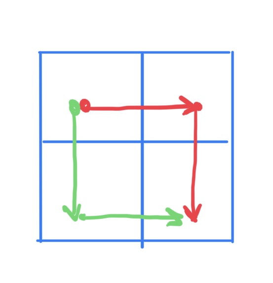
For example there are 2 ways to traverse a 2x2 array.

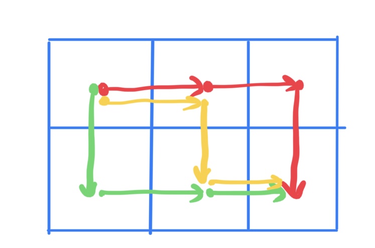
And there are 3 ways to traverse a 2x3 array.

Similarly there are 70 ways to traverse a 5x5 array.

This problem breaks down to the following top-down recursive structure. There is only one way to traverse an m x 1 array and one way to traverse an 1 x n array. For all other m x n arrays the number of ways is the sum of ways for (m-1) x n and m x (n-1) arrays.

ways :: Int -> Int -> Int 
ways 1 _ = 1 
ways _ 1 = 1 
ways m n = ways (m-1) n + ways m (n-1)

Let’s try it in ghci.

λ> :{
*Main| ways :: Int -> Int -> Int 
*Main| ways 1 _ = 1 
*Main| ways _ 1 = 1 
*Main| ways m n = ways (m-1) n + ways m (n-1)
*Main| :}
λ> ways 2 3
3
λ> ways 2 2
2
λ> ways 2 3
3
λ> ways 5 5
70

The bottom-up way of solving this problem is by initializing a 2D array A of size m x n for storing subproblem results. So, entry A[i][j] will contain the number of ways for traversing an array of size (i+1) x (j+1). This way the final result of our problem will be the entry A[m-1][n-1] and the entries are filled as A[0][_] = 1, A[_][0] = 1, and A[i][j] = A[i-1][j] + A[i][j-1].

In Python we can implement this as follows.

def number_of_ways(n, m):
    A = [[0]*n for _ in range(m)]
    for i in range(m):
        for j in range(n):
            A[i][j] = 1 if i == 0 or j == 0 else A[i-1][j] + A[i][j-1]
    return A[m-1][n-1]

In Haskell we can implement the same idea using Lists! The key is that laziness allows us to create a data structure using itself. We will compute the dynamic programming table row by row starting from the first row that is [1,1...,1]. Subsquent rows can be computed using the previous row (A[i-1][j]) and the row being computed itself (A[i][j-1]). Once this table is computed the result is the value of the last cell (A[m-1][n-1]).

numberOfWays :: Int -> Int -> Int
numberOfWays m n = last $ last table -- Result is the value of the last cell
    where
        -- table is computed as first row [1,1,..,1] followed by subsequent 
        -- rows. Each subsequent row requires the previous row for its 
        -- computation. We get the (m-1) previous rows by performing list 
        -- comprehension over the table itself.
        table :: [[Int]]
        table = replicate n 1 : [ row prev | prev <- take (m - 1) table ]
        -- row function computes the next row of the table.
        -- The next row starts with 1 (A[i][1]) followed by entries that 
        -- are the sum of the entry directly above it (A[i-1][j]) and the 
        -- entry left to it (A[i][j-1]). These entries are provided by 
        -- a list comprehension over the row being computed and the tail
        -- (because the first entry is always 1) of the previous row.
        row :: [Int] -> [Int]
        row prev =
            let r = 1 : [ left + top | (left, top) <- zip r (tail prev) ]
            in r

This implementation is very quick in practice and easily competes with traditional implementations in traditional languages.

This approach easily extends to dynamic programming problems of all sorts. If you need to lookup results to subproblems at arbitrary locations then you can consider using Vectors instead of Lists. You can generate Vectors lazily using the generate function. Let’s see this in action using another example problem.

Number of score combinations

In this problem we have to compute the number of combinations of individual plays/points that sum up to a given score. For example, there are 4 ways to combine plays/points from [2, 3, 7] to create a score of 12. These ways are -

• 2 x 6,
• 2 x 3 + 3 x 2,
• 3 x 4, and
• 2 x 1 + 3 x 1 + 7 x 1.

The top-down recursive structure of this problem is straightforward. There are -

• no ways to form a score with no plays,
• no ways to form a negative score,
• one way to form a score of zero, and
• the sum of number of ways to form the score without using the first play and number of ways to form the score using the first play at least once.

numCombs :: Int -> [Int] -> Int 
numCombs _ []        = 0 -- No ways as no plays available
numCombs score plays 
  | score < 0  = 0 -- No ways to form a negative score
  | score == 0 = 1 -- One way to form a score of 0 (use no plays)
  | otherwise  = 
        numCombs score (tail plays)         -- Ways to form the score without the first play
      + numCombs (score - head plays) plays -- Ways to form the score with the first play used at least once

A bottom-up approach is to create a table A of size (length plays) x score where A[i][j] is the number of combinations that sum up to a score of j using the first i plays. Then our final result will be the value of A[length(plays)][score].

In Python we can implement this as follows.

def num_combs(score, plays):
    m = len(plays)
    n = score
    A = [ [0]*(n+1) for _ in range(m+1) ]
    for i in range(m+1):
        for j in range(n+1):
            if i == 0:
                A[i][j] = 0 
            elif j == 0:
                A[i][j] = 1
            else:
                p = plays[i-1]
                A[i][j] = A[i-1][j] + (0 if j < p else A[i][j-p])
    return A[m][n]

Since we need A[i][j-p], where p is known only at runtime, for computing A[i][j], we’d be better of using Vectors over Lists in our Haskell implementation as Vectors allow efficient lookups at arbitrary indices. So, our table will be of type [Vector Int]. As before, the table will be computed lazily using itself and each vector in the table will be computed using the previous vector in the table and the vector itself.

numCombs :: Int -> [Int] -> Int
numCombs score plays = V.last $ last table -- Last entry in the table i.e. A[m][n]
    where
        -- The first row in the table is [0,0,..,0] as there are no available 
        -- plays. Row i is computed using its previous row (i-1) and the ith
        -- play.
        table :: [Vector Int]
        table = V.replicate (score + 1) 0 : (uncurry row <$> zip plays table)
        -- Next row is a Vector whose first entry is 1 followed by entries 
        -- computed using entries from the previous row (A[i-1][j]) and 
        -- already computed entries in the same row (A[i][j-p]).
        row :: Int -> Vector Int -> Vector Int
        row p prev =
            let
                r      = V.generate (score + 1) cell
                cell 0 = 1
                cell j = prev V.! j + if j >= p then r V.! (j - p) else 0
            in r